
In this post I describe the ideas behind Samsara a real-time analytics system. It as a walk through its design principles, and the decision behind the architecture.
Table of contents:
- Simple.
- Real-time.
- Aggregation “on ingestion” vs “on query”.
- Samsara’s design overview.
- Kafka.
- Samsara CORE.
- Why should you choose Samsara.
Simple. #
“The price of reliability is the pursuit of the utmost simplicity.” (Tony Hoare)
When I designed this system I had very hard timeline constraints. In six weeks we went from a POC in my laptop to a scalable, fault-tolerant production environment with just two people doing everything: design, development, testing, operations, monitoring and production support. With such timeline, I had to keep things very very simple.
The decision was to only use systems which were easy to setup, easy to understand, easy to debug, easy to maintain and which didn’t require a lot of time and effort in low-level fine tuning.
The choice of the language was easy, most of the tooling picked was on the JVM, and Clojure is a very good choice when the system is primarily data oriented. Its properties of immutable, functional, LISP dialect made it an excellent choice for this project. Most of all, the ability to do REPL Driven Development allowed us to cut the development time enormously maintaining fairly good quality.
Another important aspect was to be able to debug the system easily. Again the REPL came useful a few times providing the possibility to connect to a running system and inspect its state. Additionally, the ability to easily inspect the data at every stage was a paramount capability. Rushing the implementation so quickly would cause possible defects which could be anywhere in the system, so designing for human-fault tolerance was another property we tried to bake in the original design. Storing the raw data in verbatim in deep storage, ability to safely re-process the data, possibility to tear down one part of the system without losing events have been factored in the design from the beginning.
The real-time processing part was the big question. Loads of frameworks were available at the time. Things like: Storm, Spark Streaming, Samza, Flink were widely used, Onyx was a new player in this field. Yet, some had complicated processing semantics to learn, required complicated clusters setup, spend time on tuning topologies and some of them were mandating specific application packaging requirements.
We decided to start simple. The fundamental idea was to encapsulate the stream processing into a (Clojure) function which was taking in input a stream and producing a new (richer) stream as output.
With such approach we could have picked any of the more established stream processing systems later on and use it as scalable execution environment as the semantic of stream processing were encapsulated in our core; but to begin with we wrote our own Kafka consumers.
This choice became fundamentally important later on as it forged the basis for deciding how to scale the system, providing strong guarantees (ordering) for event processing and high data locality.
Real-time. #
Users of Samsara want to be able to see changes in metrics as they happen. Providing speed at scale was an important goal. Samsara provides “Real Time” Analytics, but how much “real time” is depends on various factors.
Samsara is not aiming to provide milliseconds or microseconds latency. It is more what normally is called near real-time and it ranges from sub-seconds to a few seconds of end-to-end latency. The good thing is that the latency is tuneable.
What does it mean to have tuneable latency?
In such systems you can typically trade latency for throughput. Which means that if you accept to have slightly longer latencies, you can gain in system throughput. This is simply achieved by packing more events in batches. However if you need shorter latencies you can configure Samsara to sacrifice some of the throughput.
In most of real life projects the throughput is not a variable that you can control, you have a number of users which will send a number of events and the system has to cope with it. So if we lock the throughput dimension, there is another dimension which can be influenced, and it is the amount of hardware necessary to deliver a given throughput/latency value.
Ultimately in a cloud environment the amount of hardware used reflects the infrastructure cost, in such environment you trade latency for service cost.
[~] You can trade latency for throughput or less hardware..
Aggregation “on ingestion” vs “on query”. #
The design of analytics system broadly divides in two large categories: the ones who aggregate data during the ingestion and the ones who aggregate data at query time. Both approaches have advantages and drawbacks. We will try to see how these systems do work and what are the key differences to better understand why a particular solution was picked in Samsara.
Aggregation on ingestion. #
The following image depicts what commonly happens in systems which perform aggregation on ingestion.
[~] Upon ingestion of e new event, counters are updated in memory.
On the left side we have the time flowing from top to bottom with a number of different events sent to the system. The strategy here is to split the time continuum in discrete buckets. The size of the buckets depends on your system requirements. These buckets are often called windows as well.
Let’s assume we want to know the average number of events over the last 3 seconds.
For this we need to create windows of 1 second each in our ingestion layer. Every bucket has a timestamp associated so that when we receive a event we can look at the event’s timestamp and increment the counter for corresponding bucket.
As the time flows, we will receive a number of events and increment the buckets. Buckets typically are stored in memory for performances reasons. After a certain period of time we will have to flush these in-memory buckets back to a storage layer to ensure durability and free up some memory for new buckets.
With this pretty simple approach there is already a number of difficult challenges to address. For instance how often will we flush the buckets to the durable storage? If we do it too often we will overwhelm the storage with loads of very little operations. On the other side, if we decide to keep in memory for too long we incur the risk for running out of memory or losing a number of events due to a process crash.
Additionally, how do we manage events which arrive late? If they arrive while we still have the corresponding bucket in memory, we can simply increment the corresponding counter. However, if we have already flushed the bucket to the durable storage and we have freed up the memory we will be left with no corresponding bucket in memory.
There are several strategies to deal with late arrivals and there are several papers which explain benefits of the different strategies. Whatever decision we take these are hard problems to solve in a reliable and efficient manner.
Once data is flushed to the permanent storage is becomes ready to be queried. Some systems allow to query also the in-memory buckets at the ingestion layer to shorten the latencies. The query engine will have to select a number of buckets based on the query parameters and sum all counters. At this point it is ready to return the result back to the user.
If you think that this was complicated just to get the average number of events, just sit tight, there is more to come.
Now when I’ve got the overall number of events, as a user, I realize that I need to understand how this value breaks down in relation to the type (shape) of events I’ve received.
To do so, one bucket per second is not enough. We need a bucket per second per type of event. With such buckets structure I can now compute not only the total number of events per second, but also the number of stars per seconds, for example.
There is more. What if, what I really wanted was the number of red stars per second. Well, we have to start from scratch again, this information is not available in the current information model because we took the raw events, we aggregated them and discarded the original events in favour an aggregated view only.
In order to compute the number of red stars per second we need to go back to our information model and duplicate all buckets for every type of colour we handle.
Number of buckets explosion. #
The image below shows the difference between the three queries on the same events and the buckets required to compute them.
[~] The number of buckets explodes for every new dimension to explore
You can easily see how, even in this very simple example, the number of buckets and the complexity start to explode exponentially for every dimension that we need to track.
For example just for this simple example, if we want to be able to run query across this data and retain 1 year worth of data we will need to create a bucket for every second in a year (31M circa), however querying across several weeks or months can become prohibitive due to the large number of small buckets to lookup. A common strategy is to roll small buckets up into larger one creating aggregated buckets at for minutes, hours, days and so on. By doing so, if I’m requesting the number of events across the last 3 days I can just aggregate last 3 daily buckets, or mix daily buckets with hours, minutes and seconds to get finer granularity. So if I need to query across last 3 months I have a significant smaller number of buckets to look up.
However this has a cost. In this picture there is the breakdown of how many buckets will be required to be able to flexibly and efficiently query the above simple example across 1 year.
[~] The number of buckets required even for simple cases is huge
As you can see we need to keep track of 32 million buckets just for 1 year worth of data, and this just for the time buckets, now we have to multiply this figure for every dimension in your dataset and every cardinality in each and every dimension. For this basic example which only contains 2 dimensions: the event type (4 categories) and the colour (2 categories) we will require over 256 million buckets, and above all we still haven’t stored the event itself.
Luckily there is another way.
Aggregation on query. #
If we consider the same situation with a typical aggregation on query architecture we see a different story.
Again on the left side we have time flowing from top to bottom, and a number of events reaching the system. This time we consider the time continuum as fluid as the reality, no need to create discrete buckets. As we receive an event, in ingestion we can process it straightaway. While in the previous scenario we had to be mindful of the number of dimensions, here we are encouraged to enrich each event with many more dimensions and attributes and make it easier to query.
Each event is processed by a custom pipeline in which enrichment, correlation and occasionally filtering, take place. At the end of the processing pipeline we have a richer event with more dimensions possibly denormalised as we might have used some internal dataset to join to this stream. The output goes into the storage and indexing system where the organisation is radially different.
[~] Upon ingestion of e new event, we enrich the event and store into information retrieval inverted index.
First major difference is that the indexing system stores the event itself. Then it analyses all its dimensions and creates a bucket for each property. In this bucket it adds a pointer back to the original event.
As the picture shows the bucket for the color “red” is pointing to all red events in our stream, and as more red events arrive they are added to this bucket. Same thing happens for the “yellow” events and for the different shapes. Virtually, also the time can be considered in a similar way, although the time is most system is considered a “special” dimension and it is used for physical partitioning. But for the purpose of this description we can consider pretty much in the same way.
These newly created buckets are just sets and every set just contains the ids of the events which have that property. Now if we are looking for all events in a specific timeframe, all we need to do is to take all these sets (buckets) with a timestamp within the range and perform a set union.
Now if we want to know all “red” events for the same timeframe, we do a union of the sets within the time range and an intersection of the resulting set with the “reds” set. There are plenty of optimisations to this high level view but the idea stays the same. This type of index structure is called Inverted index.
Because the aggregation happens at query time, the handling of events which arrives late is no different than the normal events. They get processed in the same way, enriched and stored like any other event. As they are added to the corresponding set for each dimension they are directly available for query and accounted in the correct aggregations.
Which approach is best? #
Both approaches have advantages and drawbacks. Which one you should choose really depends on the use you are going to make of the data.
The aggregation on ingestion offers good performances even for very large datasets as you don’t store the raw data-points but only aggregated values. However a problematic point is that you have to know all the queries you will run ahead of time. So if you have a small fix number of queries which you have to serve continuously then that’s a optimal approach.
In the projects I’ve been working on, I was looking for a system which would be flexible and support interactive and fast data exploration. In other words you couldn’t predict ahead of time all or most of the queries which would be performed over the data. In such cases aggregation on ingestion is the wrong approach. The combinatorial explosion of dimensions and values would make the ingestion too slow and complicated. To perform arbitrary queries on any of the available dimensions you need to store the original value and prepare your storage for such case.
If query flexibility is what you are looking for, like the ability to slice and dice your dataset using any of the available dimensions then the aggregation on query is the only solution.
Nowadays, most of the real-world systems have a mixed approach, but the difference is still evident when looking on how the storage layer is organized.
Samsara’s design overview. #
In Samsara we focus on agility and flexibility. Even with datasets of several billion events we can achieve very good performances and maintain the interactive query experience (most of the queries last less than 10 seconds).
Let’s see how did we manage to implement the “aggregation on query” approach with large scale datasets.
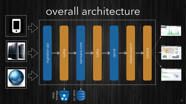
[~] Samsara’s high-level design.
On the left side of the diagram we have the clients which might be a mobile client, your services or websites, or internet websites pushing the data to a RESTful endpoint.
The Ingestion-API will acquire the data and immediately store it into Kafka topics. The Kafka cluster will replicate the events into other machines in the cluster for fault-tolerance and durability.
Additionally a process will be continuously listening to the Kafka topic and as the events arrive it will push the data into a deep storage. This can be something cloud based such as Amazon S3 or Azure Storage, a NAS/SAN in your datacenter or a HDFS cluster. The idea is to store the raw stream so that no matter what happens to the cluster and the processing infrastructure you will always be able to retrieve the original data and reprocess it.
The next step is where the enrichment and correlation of the data happens. Samsara CORE is a streaming library which allows you to define your data enrichment pipelines in terms of very simple functions and streams composition. Stream processing shouldn’t be a specialist skill, but any developer which is mindful of performance should be able to develop highly scalable processing pipelines. We aim to build the full processing pipeline out of plain Clojure functions, so that it is not necessary to learn a new programming paradigm but just use the language knowledge you already have.
For those who don’t know the Clojure programming language, we are considering to write language specific bindings with the same semantics.
Implementing stateless stream processing is easy. But most of the real world applications need some sort of stateful stream processing. Unfortunately many stream processing frameworks have little or nothing to support the correctness and efficiency of state management for streams processing. Samsara’s leverages the amazing Clojure’s persistent data structures to provide a very efficient stateful processing. The in-memory state is then backed by a Kafka topic or spilled into a external key/value store such as DynamoDB, Cassandra etc.
The processing pipeline takes one or more streams as an input and produces
a richer stream as an output. The output stream is stored in Kafka as
well. Another component (Qanal) consumes the output streams and
indexes the data into ElasticSearch. In the same way we store the raw
data we can decide to store the processed data as well in the deep
storage.
Once the data is inside ElasticSearch it is now ready to be queried. The powerful query engine of ElasticSearch is based on Lucene which manages the inverted indexes. ElasticSearch implemented a large number of queries and aggregations and it makes simple even very sophisticated aggregations.
The following picture shows the list of aggregations queries which ElasticSearch already implemented (v1.7.x) and more will come.

[~] ElasticSearch available aggregations (v1.7.x).
Once the data is inside ElasticSearch you get all the benefits of a robust and mature product and the speed of the underlying Lucene indexing system via a REST API. Additionally, out of the box, you can visualize your data using Kibana, creating ad-hoc visualizations, dashboards which work for both: real-time data and historical data as both are in the same repository.
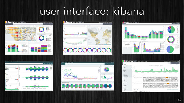
[~] Kibana visualizations (from the web).
Kibana might not be the best visualization tool out there but is a quite good solution for providing compelling dashboards with very little effort.
Cloud native vs Cloud independent. #
The discussion around cloud native architectures with their benefits versus the drawbacks is always a hot topic while designing a new system. Advocates from both sides have good reasons and valid arguments. Cloud native is usually easier to operate and scale, but with the risk of vendor lock-in. Cloud independent has to rely only on basic infrastructure (IaaS) when running on a cloud and not use any of the proprietary PaaS services. With Samsara we went a step further. We composed the system with tools which have a cloud PaaS counterpart.
Kafka, Amazon Kinesis and Azure EventHubs try to solve the same problem. Similarly Cassandra, Riak, DynamoDB, Azure Table Storage are again very similar from a high level view. So while designing Samsara we’ve took care of not using functionalities which were not available in other platforms or which couldn’t be implemented in some other way.
The result is that the system can preserve some guarantees across the different clouds and even provide the same functionality when running in your own data-center.
The next picture shows some of the interchangeable parts in Samsara’s design.
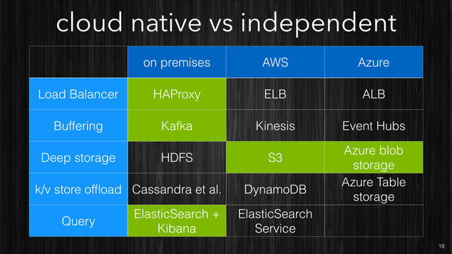
[~] Green parts are available as of 0.5, the other ones soon to come.
Cutting some slack. #
One design principle I was very keen to observe was to build around every layer some fail-safe. In this case I’m not talking about the fault-tolerance against machine failures, but specifically fail-safe against human failures. If you have ever worked in any larger project you know that failures introduced by humans mistakes are by large the most frequent type of failures. The idea of adding some sort of resilience against human mistakes is not new. The old and good database backup is probably one of the earliest attempt to deal with this issue. For many years, while designing new systems, I tried to include some sort of fail-safe here and there, but I wasn’t aware of a appropriate name for it. so when people were asking why, my short answer was something like: "… because, you know; you never know what can go wrong". It wasn’t until 2013 when I watched Nathan Marz talk on “Human Fault-Tolerance” which it came clear to me what was the pattern to follow. In the same way we try to take into account machine failures, network failures, power failures etc in our design we should also account for human failures.
In the talk, Nathan illustrates principles which, if applied, could be treated as general pattern for human fault-tolerance. The general idea is: if you are building a data system, and you build upon immutable facts, then storing the raw data, you can always go back and rebuild the entire system based on the raw, immutable facts plus the corrected algorithms. This really resonated with what I was trying to do.
Samsara encourages to publish small essential facts. By definition they are always “true”. Samsara stores them in durable storage so that no matter what happens later, you always have the possibility to go back and reprocess all the data.
Samsara cares also to make it easy to rebuild a consistent view of the world, so it gives you support for publishing external dataset as streams of event as well. Finally we avoid duplicates in the indexes which could be caused by re-processing the data by assigning repeatable IDs to every event, at the cost of some indexing performance loss. This is a deliberate choice, and it has is foundation in the concept of human fault-tolerance.
There are many other little changes which have been made to support this idea I hope you will agree with me that the system is overall better with them.
Kafka. #
Samsara’s design relies a lot on Kafka primitives. For this reason I’m going to quickly introduce Kafka design detailing why and how we use these primitives to build a robust system for our processing infrastructure.
Apache Kafka is a fast, fault-tolerant, append-only distributed log service. At its core there is the log structure. The log contains messages, every message has an offset, a payload and optionally a partition-key. The offset is a monotonically increasing number and can be utilized to identify a particular message in a specific log. The payload, from Kafka point of view, is just a byte array, which can have a variable size. The partition key is specified by the producer (sender) together with the message’s payload and it is used for data locality (more on this later).
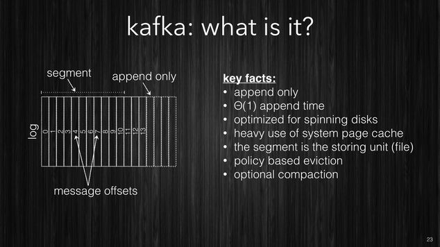
[~] The log structure of Kafka.
The log is not a single continuous file, but is divided into segments and every segment is a file on disk. The consumer (reader) chooses which messages to read, and because once written log never changes (just appends new records), the consumer doesn’t need to send acknowledgments, for the messages which it consumed back, to the server but it needs only to store what was the offset of the last consumed message.
Kafka has the concept of topics. Topics are used to divide messages for different domains. For example a topic called “users” could contains users updates, while a topic called “metrics” could contains devices sensors reading or services events. Topics are divided into partitions, and every partition is just a log. Topics can have multiple partitions and they are replicated on multiple machines for fault-tolerance.
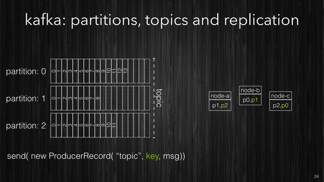
[~] A topic is composed of partitions (logs) and replicated across the cluster.
When a producer sends a message to a topic it specifies the topic name,
the message payload and optionally a partition-key. The broker,
to decide which partition must store the given message, hashes the
message-key and based on the hash fixes a partition. This is a very
important aspect as all messages which contain the same partition
key are guaranteed to be in the same partition. Such data locality is
very important to implement aggressive caching and perform stream
processing without requiring coordination. In Samsara we use the
sourceId as partition key. The sourceId is typically and
identifier of the agent or device which is producing a event. So it
means that all messages sent by a particular source will always end up
in the same partition, therefore it guarantees a total ordering of the
messages. If the partition key is not given (or null) then a random
partition is picked.
All partitions and replicas are spread across the cluster to guarantee high-availability and durability. Every partition has one and only one partition leader across the cluster at any point in time, and all messages are sent to the partition leader.
Kafka offers policy based evictions of three kinds: based on time, on size and a special eviction called compaction
[~] Kafka eviction policy: compaction.
The time based eviction deletes messages beyond a configurable amount of time. For example you can configure Kafka to retain all messages for a given topic for one week. Once the week is past messages are automatically deleted.
The size based eviction deletes the oldest messages when the total size of a topic exceed a given size. For example you can configure Kafka to keep at most 2TB of data for a given topic.
The compaction based policy is quite interesting. The compaction agent only works on non-active segments. For every message in older segments, it looks at the partition key and it takes last message for every partition key. Like in the picture, partition keys in messages are represented by the different colors, only last message for every partition-key is copied into a new segment and the old one is then removed. For example if you have three updates from “John” and two from “Susanne” then the compacted log will contain only two messages: last message from “John” and last message from “Susanne”.
This type of compaction is very useful when messages represent state changes for a given key. Similarly to a transaction log of a database, where last change is last state. If you have such situation then you can use this type of compaction to efficiently store the state changes by key, and have Kafka cleaning up the old copies for you automatically. To rebuild the state all you need to do in to apply the state of last message for every key.
Samsara processing CORE. #
Now that we have seen how the fundamentals parts of Kafka do work we can see how Samsara CORE leverages them to produce a high throughput scalable processing system.
Firstly the CORE idea is that your stream processing is just a function which takes in input a topic and produces the output into another topic. In this context we will refer to topics as streams, and since streams are potentially infinite, then the processing function has to be able to process an unbounded stream, streams get chunked as the data arrives and every chunk will contain one or more events.
[~] Samsara CORE processing.
The processing function can essentially do one of these three operations:
- filtering: where given one event it decides whether this particular event isn’t of interest for the system and it drops it.
- enrichment: where a single event is transformed and new dimensions/properties are added.
- correlation: where the relation between events can produce one or more completely new events.
Filtering. #
This is the simplest processor you can have, given an event you can
decide whether to keep the event (return it) or drop it (return
nil).
ƒ(e) -> e | nil
When working with systems which do aggregation on query, you typically want to store all events you receive, so isn’t very common to have loads of filters. However in your processing you might correlate two or more simpler events to generate new richer high level events which are both: more complete and contain all information which you have on the simpler ones. In such cases you often might want to drop the simpler ones as they are less informative and harder to query than the high level ones. You can build a filtering function from a conventional predicate functions.
Enrichment. #
The enrichment functions are the most common. It is here where you can
add all the additional information that you know about a particular event.
The enrichment function is a function which takes one event and it returns
a richer event or nil.
ƒ(e) -> e' | nil
If an enrichment function returns nil it means that it doesn’t have
any enrichment to do with this particular event. This semantic sugar
allows very idiomatic code in Clojure, and avoid accidental dropping
of events. In fact the only way you can eliminate an event is via a
filtering function.
Common uses of the enrichment functions are to add calculated
attributes, or to add additional properties from internal
data-sources. For example you might receive an event from a device
and look up in your company data-sources for the owner. Or if you
receive an event from a user with its userId you could lookup in
your user’s data-source for more information about the particular
user. Adding this information directly into the event allows you to
easily make queries based on user’s properties.
Correlation. #
The correlation type of functions allow you to produce completely new events. You typically going to use other events which you might have already seen in your processing stream to generate new events. One common example could be that your system receives events which denote the starting and the stopping of an activity and you could use a correlation function to generate one new event which represent the activity itself and its duration (Samsara has a module which provides this functionality).
The correlation function is a function which given an event can return zero, one or more events.
ƒ(e) -> [] | [e1] | [e1 e2 ... en]
Also here if the correlation function returns nil it is considered as a
no-operation (no new events are generated). One interesting aspect of
correlation functions is that the newly generated events are inserted
in-place in the stream and processed with the entire processing
pipeline like if they were received from a client. This approach
simplifies a lot the processing pipeline as you have the guarantee
that every event will go through the entire pipeline even if the
correlation function produced them mid-way in your processing.
The following image shows how the events are processed and what happens when a correlation function generates new events.
[~] The correlation adds new events in-place in the stream, like if they were sent by the client.
Composition: Pipeline. #
We’ve seen how you can organize your processing semantics into simple
building blocks like the functions which perform the filtering,
enrichment and correlation. However any non trivial processing will
require to define many of these different functions. Samsara allows
to compose these simple functions in more complex and structured
pipelines. Like the Clojure function
comp which is used to
compose many functions into one, Samsara offers a function called
pipeline which will compose filtering, enrichment and
correlation functions into a single processing pipeline.
Like the picture below shows, pipeline can take many different
functions (with different input/output shapes) and compose them into a
single function which will be the equivalent of all single functions
executed one after the other one in the given order.
[~] Samsara allows you to compose your stream processing from very simple building blocks.
Samsara also offers tools to visualize a pipeline and produce a flow diagram with the different functions.
Enrichment, filtering, correlation and the ability to compose them
into pipelines are provided as a library called moebius which is
part of Samsara. I’ve designed this as a separate library so that your
processing pipelines can be designed, built, and tested, in
complete isolation using just pure functions without requiring a
running cluster or complex testing infrastructure. Once your
processing pipelines are build you can test them by providing events
directly and verifying the expected output. No mocking required, just
pure functions.
State management. #
So far we have seen how to do stateless stream processing which is the easiest form. However most of real-world projects require more complex processing semantics which often are powered by transitory computational state.
Some stream processing frameworks have little or nothing to help developers to get stateful stream processing right. Without support, developers have little or no choice to use their own custom approach to state management.
In this section we are going to see various approaches used by different frameworks and then we are going to explore Samsara’s approach.
The first approach is to store your processing state using an external DB cluster, typically a k/v-store such as: Cassandra, Dynamo, Riak to name a few.
This is the easiest approach but also the weakest one as well. Even if your database is well tuned, as the processing rate grows, it is likely to become a bottleneck in your processing. After a certain stage it will become harder and harder to scale your stream processing system due to the database. Database are much harder to scale, even system like Cassandra which scale very well, sooner or later will become the dominant part in your execution time. To push the database beyond certain points requires more nodes. While your stream processing will be quite fast with a modest number of machines, your DB, likely will require huge clusters.
The following picture shows processing nodes connecting to an external k/v-store to persist their transitory state.
[~] The simplest approach (not good) is to use external k/v-store.
One additional challenge in case of processing failures is that the state can get easily out-of-sync. For example the processing node might have stored successfully the data into the k/v-store, but it failed to checkpoint it’s own progress.
The second approach is to use the data-locality offered by Kafka, and the guarantee that all events coming from a given source will always be landing in the same partition. Keeping this important fact in mind, it is possible to use local (to the node) caches such as: Redis, Memcache and RocksDB to name a few.

[~] A local cache offers better latency and better scalability profile.
Because every node is independent from the others it is much easier to scale. While in the external database the read/write latencies are in the order of 1-10ms, with the local cache the latency is typically around 100𝛍s-2ms. However you still have to incur the serialization and de-serialization costs on every read/write.
In Samsara we designed a in-memory k/v-store using the fabulous Clojure’s persistent data structures to store the state. To guarantee durability we back changes in into a Kafka topic which is used to store the state only. Samsara’s k/v-store produces a transaction log of all the changes made to the in-memory data and when Samsara writes the output of the processing into the output topic, it writes the changes to the state into the kv-store topic.
[~] Samsara’s kv-store is in-memory and in-process.
The use of Clojure persistent data structures makes the k/v-store friendlier to the JVM Garbage Collection, and being in process there is no serialization costs of every read/write. The typical latencies for Samsara’s k/v-store are 100ns read, 1𝛍s write, additionally every thread has his own thread-local k/v-store which eliminates contentions and the need of coordination (locks), overall it has just better data locality for your process. If your processing state is way bigger than the available memory on your nodes you have two options: the first one is to add more nodes and distribute the processing across more partitions. If this isn’t viable for solution cost-wise you can have the k/vs-store to spill into an external db cluster. Such solution is still better than making db lookups for every event as the k/v-store will only go to the external db in case of a cache-miss and will only store when the entire batch has been processed (not for every single event). Considering that events from a given source tend to arrive in batches due to the client buffering it is easy to understand the advantages of this approach compared to the first approach we discussed. If you are really sensitive to the latencies the only solution is to add more nodes.
Finally, let’s see how Samsara is fault tolerant in respect to the state management. We said earlier that the k/v-store we use is in memory, so what happens if a node dies?
The following picture illustrate what are the steps in such case.
[~] Samsara’s state management fault tolerance.
- The system is running and all nodes are consuming their own share of partitions.
- As events are processed the output is written into the output topic and the state changes are persisted into the k/v-store topic.
- The “node 2” dies due to a machine failure. The processing of that partition stops. In memory state is lost.
- After some time the machine comes back alive.
- Samsara initializes the k/v-store using the transaction-log in its own topic.
- After the full state is restored, the node starts to process events from the partition as before, with the exact state that was left before the failure.
To avoid that the k/v-store topic becomes huge impacting the restart time we use the Kafka’s compaction feature for this topic. So over time only latest copy of the keys will be kept.
This pattern is used by other processing systems notably Apache Samza and the very new Kafka-Streams.
This is the way Samsara maintains state and offers a support for the stateful stream development directly in its core. All functions which process events that we seen earlier such as filtering, enrichment and correlation they all have a stateful variant as well. In the stateless processing they only accept an event, if you need stateful processing, then they will accept the current state and the event.
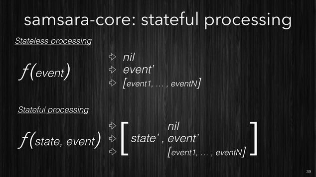
[~] Samsara’s stateful processing functions.
Stateful functions and the stateless ones can be mixed in the same
pipeline. The pipeline function takes care of passing the state to
these functions which requires one and only the event to the stateless
ones.
Earlier we said that the stream processing is a function of the input stream to produce an output stream, now for you stateful stream processing we can say that is a function of the input stream and the state topic, to produce output stream and an update state topic.
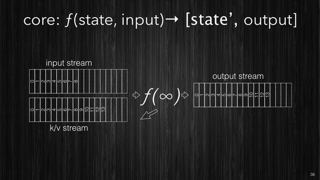
[~] Samsara’s stateful processing representation.
Finally if you have internal data sources which you want to use to
enrich your data you can provide them as a stream and Samsara will
convert them into k/v store. This is often useful when you have
internal data-source such as your users database or your products
catalog etc which you might want to join with incoming events enriching
them with additional dimensions.
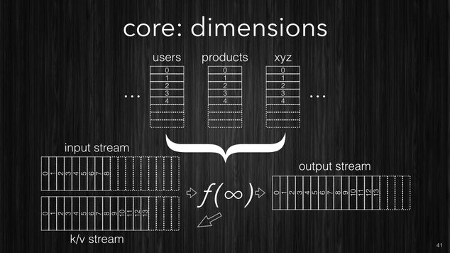
[~] Samsara support external datasource as streams.
These dimesions are available in your processing functions as globally accessible in-memory k/v-stores, and because they are just streams of changes, they can be updated while the application is running without downtime.
Why should you choose Samsara. #
I designed Samsara because I think that although many systems allow you to do stream processing, the stream processing part is just a small part, albeit important, of delivering a system which provides real-time analytics. Samsara is a full stack. We provide clients for your devices or your services, we provide a way to ingest the data, we provide an easy and scalable solution for events processing, a very fast storage, visualization, dashboards, and a number of built-in modules to facilitate common scenarios.
All other alternative solutions are either not providing the full stack, or they are proprietary services and very expensive solutions. With Samsara you have a open source solution that lets you keep your own data, and provides all the capabilities to build very sophisticated models.
I’ve used this system to build a real-time recommendation engine. Because the processing system is made of just plain Clojure functions and its execution model is very clear, you can easily develop extend the system to build new products or services with the same platform.
Having a real-time analytics system as part of your services is invaluable. You can understand how users interact with your services as it is happening. You can use it for general analytics, you can use it as a Multi Variant Testing (MVT) system, you can use it for monitoring KPIs and in many other different way.
Many BI solutions rely on batch systems which have incredibly high latencies, Samsara is performing incredibly well in this space. Much of the merit has to go to ElasticSearch for this.
In the following picture there is a performance comparison which I made for one of my clients. It was performed using the same data on the same cluster size with similar machines. The first query shows the time it took Hadoop + Hive to perform a simple filtering query with aggregation across 1.8 billion records. The same query was then performed with Spark + Hive and ElasticSearch.
[~] Query performance comparison.
You can see the incredible difference, 6 seconds against the 2 hours for Hadoop. Samsara with ElasticSearch enables an interactive data exploration experience that other products are just not able to provide.
I hope the reader will find this description interesting and that it helped to shed some light on Samsara’s internals. Try the open source project and visit the website.